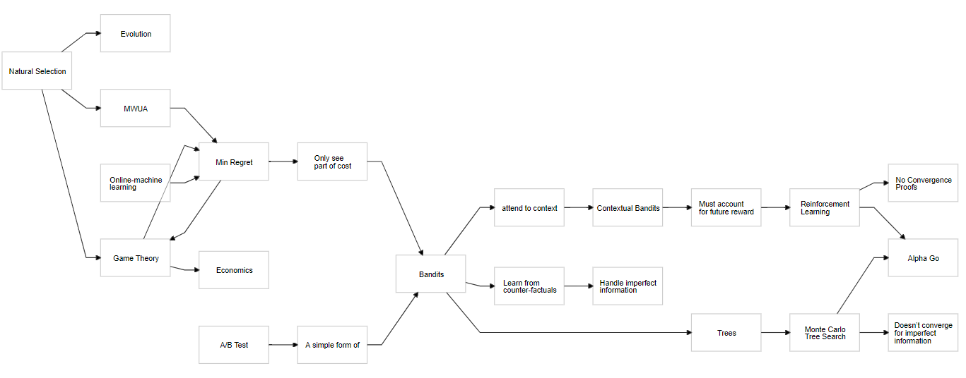
In the image above, I've sketched how one can show that evolution, game theory and learning are related. While I'll not talk about natural selection today, I'll discuss how ideas from game theory can be given an easier footing from within the context of computational learning theory. A future post will discuss evolution from the min-regret framework so it's worth following the ideas presented here. Topics: AI economics (why capitalism is intractable), games, learning algorithms. I must apologize—ideally, there should have been interactive demos but alas, I hadn't the time for that.
The Nash Equilibrium (NE) is a solution concept for games. Games are a framework which prescribe how to behave and coordinate optimally in a given situation, assuming some way of ranking outcomes (utility) and effectively infinite computation (among other unreasonable things). Okay to be fair, people have recently been looking into how to operate under the constraints of resource limitations. The min-regret framework has informed some of that work.
A NE can either be pure (where you play only one strategy) or mixed (where you randomize over your strategy set). A strategy is essentially a look up table (or algorithm) telling you how to behave at all decision points. Not all games have a pure NE but all (finite) games have at least one mixed NE. At a NE, each player gains no utility from switching to a different strategy profile. Although highly celebrated, NEs are actually rarely practical for several reasons. They inhabit the PPAD complexity class (which are conjectured to be intractable), work best in 2 player zero sum (or other simple) scenarios (there can only be one winner) and will not necessarily find a fair solution concept. The utility of the the solution concept for general sum games is also questionable. Finally, although they are in some sense optimal, they do not necessarily provide the "best" results. In particular, for 2 player 0-sum games, NEs have zero expectation.
As an example, consider Rock Paper Scissors. The mixed NE for this game is to randomize evenly: play one of the pure strategies of always playing one of rock,paper or scissors with 1/3 probability (to be clear, an example of a pure strategy in this game is to always play rock).
If you always play: 📰 then I can switch to a strategy of always playing ✂. It you play a strategy like [👊,70% ;📰, 10%; ✂, 20%; ] then I can play the pure strategy of [📰, 100%] and perform optimally against you. This is because 70% of the time I win, 10% of the time I tie and only 20% of the time am I losing. You can expect to lose -0.5 in expectation (this might not seem like much but on average, if we play 100 rounds and bet 5💵/round each, then I'd have taken 💲250 from you). You can check the code here, other adjustments will do worse than just playing pure paper.
let regretSum   = [|0.;0.;0.|]
let strategySum = [|0.;0.;0.|]

let rpsStratDef  = Array.zip [|Rock;Paper;Scissors|] [|0.7;0.1;0.2|] //<== These numbers can be changed. Ensure sums to 1.
let rpsStratDef2 = Array.zip [|Rock;Paper;Scissors|] [|0.2;0.7;0.1|] //<== These numbers can be changed. Ensure sums to 1.
let rpsNE = Array.zip [|Rock;Paper;Scissors|] [|1./3.;1./3.;1./3.|]
                                              //       ___________
                                              //       |                        |
                                              //can change this  \|/
train1 20_000 winner [|Rock;Paper;Scissors|] (Array.map snd rpsStratDef) regretSum strategySum
Imagine you always played 📰. Then 1/3 times you'll tie with 📰, 1/3 times you'll win against 👊, and 1/3 times you'll lose vs. ✂.
There might even be runs where it will seem like you're winning. If your goal is to maximize profit against an opponent, then NE might not be the correct strategy for games like RPS.
One thing you might try would be to learn patterns of your opponent and then playing a strategy exploiting that. The problem is this in turn always leaves you vulnerable. The opponent might know what you are doing and mislead you for a bit and then BAM, switch things up and collect some wins before your algorithm notices something is off. A NE has the advantage that even if your opponent knew what you were up to, they still could not (e.g.) take money off of you (in the long run).
Not all 0-sum 2 player games have the interesting quirk where it's impossible to lose against an optimal player. Some games punish you for taking stupid actions. Of course, stupid is relative, and some games such as poker have action spaces so complex that it's very, very difficult to know when you're being stupid. For this example we'll look at a simple extension of Rock, Paper, Scissors. We'll add another move: telephone. How to handle rewards? If we make telephone a duplicate of paper, then we end up with a game that's exactly the same as RPS save that there are now two equilibria: [👊,1/3 ;📰, 1/3; ✂, 1/3; 📠,0%] and [👊,1/3 ;📰, 1/6; ✂, 1/3; 📠,1/6]. The other aspects, where playing any mixed non-equilibrium strategy can be defeated by a pure strategy or where it is impossible to lose against an optimal player remain.
Imagine you played pure paper again. Then a NE player will either play the same mixed strategy as for RPS, with the same results or play the second NE strategy. Then: 1/3 of the time you lose against rock, 1/3 of the time you win against scissors and tie for the other two scenarios.
What if we made the telephone over-powered? That is, it ties against everything except paper, which it defeats. What's the best way to play against someone who only plays telephone and what's the equilibrium for this game?
Did you get it? Don't play paper. As long as you don't play paper then you have a zero loss expectation against a pure telephone player, which is also the pure equilibrium strategy for this game. Playing paper is the stupid action, with your loss proportional to the probability with which you play paper. In this game, it is possible to lose against an equilibrium player by playing paper.
Poker is a game like over-powered telephone, rock,paper, scissors. The optimal player only wins because there are stupid actions you can take which act essentially as donations. In our modification to RPS, it's clear that playing paper is dumb. Let's modify the game to make it a bit more complex. A slight mod to RPST such as 📠 loses to ✂ but defeats 👊 and 📰 yields a slightly more interesting result. Once again, playing paper is a stupid action but playing just 📠 means someone else can play just ✂. The NE is: [👊,1/3 ;📰, 0%; ✂, 1/3; 📠,1/3]. With some thought, you should notice that as long as we never play paper, we can't lose against an optimal player. Even playing just 👊 is fine since 1/3 of the time we defeat ✂,1/3 of the time we lose to 📠 and tie with 👊 1/3 of the time. This game has a "stupid" action but offering to play against someone out of the blue, they might not realize that paper is a trap.
The final modification will be to introduce this game: Telephone ties with telephone, Telephone loses to scissors but 50% of the time it defeats rock and 4/6 of the time it defeats paper. The game is no longer straightforward but it's a lot closer to the original RPS. The NE is [👊,1/3 ;📰, 1/3; ✂, 1/3; 📠,0%], other mixed strategies have a pure counter. A strategy like [👊,40% ;📰, 40%; ✂, 10%; 📠,10%] can be countered with [📰,100%]. The expected win rate is ~0.26. This can add up:
This time, the only way to lose against an optimal player is to include telephone in your mix. Although it seems powerful (can defeat paper ~67% of the time and 50% vs rock and only loses to scissors), in the long run it loses (playing pure 📠 has a lose rate of about -0.22). If properly presented, a player can easily be tricked into thinking that 📠 is over powered.
You can look at the code relevant to this section here.
Press Play buttonWell, I think that's about enough of rock, paper scissors. Although zero sum games are well studied, this is because they are one of the few scenarios where computing a Nash Equilibrium is tractable. There are probably not many situations that are 2 player and zero sum, and the concept of zero sum is really only sensible in the two player setting. For example, people might say that markets are zero sum in the short run but that doesn't make sense to me. Firstly, this requires that the traded currency amount is equal to the utility or the value placed by the respective traders. This need not be the case. Secondly, the game can really only be two player if we pretend that other players actions do not affect the available actions and information. This seems unlikely too. Beyond Games and Game Theory exercises, it's hard to think up scenarios that are genuinely two player and zero sum. Sometimes I think people claim zero sum as an excuse for their selfish behavior without any real understanding of what the notion entails.
Even two player general sum games can be intractable—as I mentioned earlier general sum games can have NE that are too difficult to find because finding a NE is in the computational complexity class of PPAD.
Computational Complexity seems like a subject you'd get if you combined zoology, logic and a guide on how to survive the apocalypse (let's prepare for the worst). There's a lot of taxonomical terminology with strange names that will quickly turn any onlooker dizzy. When reading about Nash Equilibria in the context of poker bots and evolution, I nodded to myself and said "ah yes of course it would be PPAD...😏". I'm still not confident in my understanding—there are lots of fine details—so will welcome any corrections.
Everyone who has heard of computational complexity has probably heard of polynomial time vs non-deterministic polynomial time (NP). By the way, the unwieldy naming of NP derives from the non-deterministic turing machine (NDTM) which is essentially a psychic computer and should not be confused with a proper probabilistic computer. NDTMs take choices in a way that is not determined by their state and solve NP problems in polynomial time by magic. Polynomial time (P) is in principle efficient but anything that scales faster than a factor of N^2 is truly stretching the meaning of efficient. Many useful algorithms are O(N^3) and unusable in practical settings. O(N log N) is about the limit of what is practically efficient (matrix x vector is O(N^2) but manages due to how well it parallelizes).
Problems that are NP-hard are not tractable to solve and their solutions are not necessarily efficiently verifiable. Problems in NP are efficiently verifiable and NP-complete problems are problems where a solution to one of them yields a solution to all other problems in NP. Of course P is in NP. NP-complete problems are NP-hard problems that are efficiently verifiable. P and NP actually deal with decision problems. My favorite description of the question of whether P=NP is whether search is equal to recognition/calculation. Since we can also view learning as a form of search, the question of whether P=NP can be seen as: Is learning ever necessary? From this frame, P=NP, even with a high polynomial (which would be to say, no, planning and learning are not needed in theory) seems somehow unnatural.
A decision problem is, if I asked "what's the shortest tour through these cities" and you replied "what?". And then I rephrased it as: "sorry, what I really not really meant to ask, is there a tour through these cities that takes less than N number of steps?" to which you said "yes" and fell silent. As you can see, decision problems are very curt and business like.
Well, a corresponding class is FP and FNP which deal with function problems. This class is more literate and actually does things, like, returning an example which satisfies my touring question. FNP has the same property as NP of efficient verification. FNP might not always return an answer so there is a subclass, TFNP, dealing with total functions which always return an answer. PPAD is a subset of that class with the further requirement that the proof gadget of totality is by a directed graph. PPAD problems are conjectured as harder than FP problems and this conjecture is borne out by a lack of any polynomial time algorithms for their solution (although there are exponential lower bounds).
This is the essence of the class PPAD: search problems whose existence of solution is guaranteed by virtue of an exponentially large directed graph, implicitly represented through an algo- rithm, plus one given unbalanced point of the graph. Many problems are known to be PPAD- complete; perhaps the most fundamental such problem is related to Brouwer’s theorem ... And it seems counterintuitive that there is always a way to telescope the search through all points of an exponentially large directed graph, to zero in the other unbalanced node, or the sink, that is sought.
Page 3 | PNAS-2014-Papadimitriou-15881-7
Many celebrated concepts of economics rely in some way on Brouwer's fixed point theorem. Actually finding this fixed point is PPAD-complete, in other words, intractable. In addition to Nash Equilibria there is also the Arrow-Debreu theorem, which tells us of the existence of a price equilibrium in free markets (under realistic conditions), where allocation of resources are pareto efficient. Pareto efficiency is a concept of "fairness" which is optimal in the sense that there is no reallocation of resources that doesn't leave someone worse off and unbalanced. "Fairness" because a pareto efficient allocation need not be what we would intuit as fair. In a scenario where you have 99/100 items and I have 1/100, any reallocation will leave one of us worse off.
Common attacks against markets include violations of perfect information, transaction costs, externalities, barriers, assumptions of convexity in preferences and so on.
However, even before looking at those utopian requirements, we find that the very concepts motivating markets require intractable computations to reach their notion of fairness. And these (Nash, Pareto, Arrow) are not even guaranteed to be fair in an intuitive sense. It's informative to contrast these computational issues of markets with those of Planned Economies—which are at least tractable in principle (but not in practice, "merely" requiring O(N^3.5) scaling with problem size). This is not to say that markets lead to worse outcomes than planned economies, merely to point out it is technically more impossible to achieve fair outcomes with them, compared to planned economies.
At this point, the concept of what an economy entails is worth revisiting given what we now know from computational learning theory. We can do better than planned or market economies.
Although the Nash Equilibrium is much celebrated, the correlated equilibrium concept is more natural in several senses. It's not just tractable but also efficiently computable to high accuracy, the dynamics of many learning algorithms converge on it (or its coarse version) and even agents acting independently can conceivably converge to its equilibrium concept. But what is it? I actually find the definition to be a bit awkward.
The correlated equilibrium is a joint (as opposed to Nash's independent) probability distribution over action profiles where, the expected utility from playing according to a drawn profile, conditioned on seeing its suggested action at least matches that of any other actions' (it is a best response). A coarse correlated equilibrium is similar except there is no suggested action to condition on—they can lead to lame, weakly dominated suggestions however. In math, a correlated equilibrium is:
\(E_{a\sim D}[u_i(a)] \ge E_{a \sim D}[u_i(x_i,a_{-i})|a_i]\)
for every action \(x_i\). For the coarse version, there is no \(a_i\) to condition on. Algorithms which minimize external regret converge on coarse equilibria whilst those minimizing swap or internal regret converge on correlated equilibriums.
More clearly, imagine there is some neutral device. This device draws from a joint probability distribution and tells each player to play according to its suggestion: a correlated equilibrium is when there is no incentive to deviate from its suggestion. These outcomes can be better than the Nash concept since CEs act on the joint space of actions while the Nash concept is very solipsistic and self-centered, looking at signals provides no information.
The example everyone gives is a traffic light signal. When it shows GO, you know the other player sees a STOP so there is no incentive to deviate. Here are some other examples I think should count, roughly in order of how well they fit: the non (now dead) Dennard Scaling portion of Moore's Law, the I give up signal in animals (such as when a dog lays on its back—it's better to think of the phenotype and not any specific instantiation as the player), functioning courts and laws, rituals/tradition (however, as self identity and values shift and change, such systems quickly induce equilibriums that are inequitable).
Regret minimizing algorithms are a class of efficient on-line (meaning learn on the go) learning algorithms which given some reward function and access to some set of experts (which can also be moves such as rock in RPS), which quickly learn what actions to take in order to minimize long term regret. External regret minimizers do this with respect to a fixed strategy while internal regreters do this with respect to any swapped set of actions. The internal regret scenario lets you say when I did this, I should have done that instead. External regret says, I did almost as well as that really good advisor.
Prediction markets let people bet on binary propositions. Imagine there was a prediction market with a layer tracking how well each bettor (expert) did. External regret could do almost as well as the best bettor and perhaps even better with randomization over all bettors, weighted according to how well they did in the past.
I believe, but am not certain, that a scenario where you could match experts to contexts: for example, a technology expert, a sports expert and so on would likely allow you to minimize something like internal regret. From this you could even extract a weighted average over hypotheses.
For more detail on regret algorithms, you can take a look at the demo code. I implement both Multiplicative Weights Update and Regret Matching.
Consider the following game: there are N people, you each choose a number between 0 and 5 and show it with your hand 🖐 on a ready signal. The winner is the person displaying the lowest unique number. The winner gets a score equal to N-1 while everyone else gets a score of -1. This makes it effectively a 2 player 0-sum game. What's the Nash Equilibrium strategy? I don't know but when I run this I get the following sequence:
Move |
Move Probability |
|---|---|
0 |
0.499 |
1 |
0.25 |
2 |
0.126 |
3 |
0.063 |
4 |
0.031 |
5 |
0.03 |
Which is a pattern of ~\(0.5^{x+1}\) but with some aliasing at the end. Simulation gives a mean utility of -0.006 ± 1.31 (regret algorithms only get within epsilon of the exact equilibrium). The distribution over means is: -0.0006 ± 0.01. This corresponds to a win ~28.8% of the time, a loss ~56.9% of the time and a tie ~14.2% of the time. This looks close to what's realistically achievable. It's also interesting that in this game it is both possible to not be able to lose (if playing against two optimal players) or lose while providing donations to a single optimal player (with two off equilibrium players).
What happens when we try for a coarse correlated equilibrium? In this, I also apply regret matching on 3 players trying to maximize utility while looking at the other players. Sometimes, an interesting strategy emerges which kind of looks like collusion in that two players end up with positive expectation (e.g. 61% win, 39% lose, 0.83 expected utility; 61% lose, 39% win, 0.17 EU) and one is guaranteed losses such that it doesn't matter what they do:
Move |
Move Probability |
|---|---|
0 |
0.395 |
1 |
0.289 |
2 |
0.132 |
3 |
0.079 |
4 |
0.053 |
5 |
0.053 |
GUESS STRATEGY2
Move |
Move Probability |
|---|---|
0 |
1 |
1 |
0 |
2 |
0 |
3 |
0 |
4 |
0 |
5 |
0 |
GUESS STRATEGY3
Move |
Move Probability |
|---|---|
0 |
0 |
1 |
0.091 |
2 |
0.091 |
3 |
0.455 |
4 |
0.182 |
5 |
0.182 |
Usually, a strategy emerges where one dominates: (e.g. 77% win, 23% loss,1.3 expected utility), another has moderate-large losses (23% win, 77% loss,-0.3 expected utility) and the last has guaranteed losses. This is surprisingly reflective of reality 😝😔
Another strategy would be if there was some device which sampled uniformly from a joint probability distribution after eliminating any ties. This would have expectation equal to the game for all, that of zero, matching the Nash equilibrium. No one would have any incentive to deviate knowing that everyone was playing according to the suggestions of the device. Note that knowing my number also tells me something about what the others saw: if I get a 2, I know that no one else received that number. Something else worth noting is that part of this game's problem is it's zero sum. If the game was not zero sum, the outcomes could sometimes be even better than Nash.
Code here:
[|for _ in 0..999 -> runRound()|]
 |> Array.groupBy id
 |> Array.map (keepLeft (Array.length>>float))
 |> Array.normalizeWeights
 |> Array.sumBy (joinpair ( * ))
 |> round 2
 |> printfn "\n=========\nWinrate of Strategy 1: %A"
This example is a simple game where two players are at an intersection. If they both GO 🚙 they both suffer a utility of -100. If one drives and the other STOPs 🛑 then the goer gets a utility of 1 and the other 0. If they both 🛑 then they both get a utility of 0. This is no longer a zero sum game. The regret matching algorithm learns the following strategy:
Move |
Move Probability |
|---|---|
A 🛑 |
0.99 |
A 🚙 |
0.01 |
This is pretty lame since there is a 0.01% chance of a catastrophic incident. The expected utility is ~zero for both players. If we try regret matching on two players that try to coordinate we get:
DRIVE STRATEGY
Move |
Move Probability |
|---|---|
A 🛑 |
0 |
A 🚙 |
1 |
DRIVE STRATEGY2
Move |
Move Probability |
|---|---|
A 🛑 |
1 |
A 🚙 |
0 |
In this scenario one player always goes and the other always stops. Thus one player gets a utility of 1 per round while the other always gets 0 but there is a 0% chance of a crash. While not ideal for one player, the situation is overall better than the Nash equilibrium strategy which has an expected utility of 0 for both players. Notice that without some way to independently and reliably coordinate, it is not possible for the pair to do better than the above.
If instead we optimize over the joint space of actions we get:
DRIVE STRATEGY
Move |
Move Probability |
|---|---|
(A 🛑, A 🛑) |
0 |
(A 🛑, A 🚙) |
0.5 |
(A 🚙, A 🛑) |
0.5 |
(A 🚙, A 🚙) |
0 |
This is a correlated equilibrium and is fair for all parties, with both experiencing a positive utility. Yet there is a sense in which this result is unsatisfying. It is rare that we can compute or even know what joint probability distribution is being sample from, to speak of how to properly compute a reward on it. But as I mentioned above, agents working independently can sometimes learn to do this.
In this (scroll down to bottom to see results) modification to the driving game, I use Multiplicative weights update with two layers of weights. The first layer of weights computes the cost of adhering to the signal or listening to an inner expert. The inner expert learns regret from playing either 🛑 or 🚙. Thus the agent has the ability to either heed the signal or do as it pleases. To make things interesting I vary the reliability of the signal. A signal with 90% reliability does as it pleases 10% of the time. In this case the agents learn to ignore the signal and settle on a strategy equivalent to when there is no signal (one always goes and the other always stops):
Agent1: ["🚦: 0.0%"; "😏: 100.0% [(A 🛑, 0.0); (A 🚙, 1.0)]"],
Agent2: ["🚦: 0.0%"; "😏: 100.0% [(A 🛑, 1.0); (A 🚙, 0.0)]"]
Sometimes however, one agent will choose to heed the signal while the other chooses to always stop:
["🚦: 0.0%"; "😏: 100.0% [(A 🛑, 1.0); (A 🚙, 0.0)]"],
["🚦: 99.44%"; "😏: 0.56% [(A 🛑, 0.4); (A 🚙, 0.6)]"]
It takes about 99.9% reliability for the agents to consistently choose a strategy that goes along with the signal, matching the correlated equilibrium.
["🚦: 99.68%"; "😏: 0.32% [(A 🛑, 1.0); (A 🚙, 0.0)]"],
["🚦: 99.72%"; "😏: 0.28% [(A 🛑, 1.0); (A 🚙, 0.0)]"]
let drive =
    function
      | (``Do 🛑``,``Do 🛑``) -> (0.,0.)
      | (``Do 🛑``,``Do 🚙``)   -> (0.,1.)
      | (``Do 🚙``,``Do 🛑``)   -> (1.,0.)
      | (``Do 🚙``,``Do 🚙``)   -> (-100.,-100.)

let getExpert signal (actions:_[]) (experts:_[]) =
    let e = discreteSample (Array.map fst experts)
    match experts.[e] with
     | (_,``Do 😏`` es) -> actions.[discreteSample es]
     | (_,``Do 🚦``)     -> signal
This result still feels unsatisfactory since one might argue that there is too much hand-holding. Therefore, in this version, I decided to make a learner that must learn how to read the signals and how to coordinate. The hand holding is minimal and typical of features in Machine learning algorithms. The system is inefficient in that it tracks all possible combinations—this is clearly untenable for more players,signals, and granularity. However, it doesn't take much work to modify the system to explore adding and removing rules in an attempt to learn a Set Cover over rules. But generally, one of the hardest parts of machine learning is getting efficient representations of large or complex state spaces.
let inline getExpert2 indicated signal (rules:_[]) =
    let cs = [|for (p,_,f) in rules do
               match f indicated signal with
                | Some c -> yield c,p
                | None -> ()|] |> Array.normalizeWeights
    let ps = Array.map snd cs
    fst(cs.[discreteSample ps])
In this model, any rule that matches the current situation is filtered to, after which weights are normalized for this reduced space. An action is taken and then a reward is used to calculate regret on only the active rules. This system is richer than all the previous and so allows us to explore an interesting few scenarios. The game is also modified as such: a player acts first and then the second player decides what to do based on what the first player does.
If we have the first player choose an action without looking for a signal and then have the second player decide based on the first the following major rule pair is arrived at:
[(1.0, "if signal=Do 🛑 && other=Do 🛑 then Do 🚙")], [(1.0, "if signal=Do 🛑 && other=Do 🛑 then Do 🚙")]
Essentially, only drive if the other driver stops. Because of how the system filters matching rules, missing values end up such that only one value is looked at but this ends up including rules which don't make sense when the full conjunction is looked at. One fix would be to include an additional state representing none, but that's not necessary for demonstration purposes. Nonetheless, the agents work around that issue and learn a useful set of rules. Sampling some interactions we see that most of the time the first car will do whatever (usually drive) and the second one will drive or stop depending on the other. We see that the situation learned is better than the experts above without access to a signal. The first player dominates but the second player still sees a positive reward.
[((Do 🛑, Do 🛑), 0.1); ((Do 🛑, Do 🚙), 0.36); ((Do 🚙, Do 🛑), 0.54);((Do 🚙, Do 🚙), 0.0)]
If we instead provide a signal for what the other will do as the light they see (the system can't reason after all), the following rule pair is matched:
[(1.0, "if signal=Do 🚙 && other=Do 🛑 then Do 🚙")],
[(1.0, "if signal=Do 🚙 && other=Do 🛑 then Do 🚙")]
And we see that their behavior is converging on a correlated equilibrium:
[((Do 🛑, Do 🚙), 0.49); ((Do 🚙, Do 🛑), 0.5); ((Do 🚙, Do 🚙), 0.0)|]
On the other hand, if we take away the ability for the agents to attend to what the other will do they will tend to learn either a set of rules that are either nearly a Nash Equilibrium or sometimes, nearly a correlated equilibrium (something I find to be surprisingly robust).
[((Do 🛑, Do 🛑), 0.97); ((Do 🛑, Do 🚙), 0.03); ((Do 🚙, Do 🛑), 0.0)]
In essence, so long as you can jointly learn to attend to signals, and so long as there is some shared memory to draw upon (history, text) then many learning agents can efficiently converge on a correlated equilibrium, bottom up. Without any top-down enforcement of joint distributions. In the absence of anything to condition and coordinate actions by, coarse equilibria (which I expect many short term—within the life of an individual—scenarios share much in common with) can be subpar.

As an example, I think the historical knowledge of Bali Rice Farmers [1], with insects and weather as the coordination signal lead to a bottom up correlated equilibrium of planting patterns.
So far (excepting the last rule based AI scenario), the focus has only been on Normal Form (no turn taking) games but the story for imperfect information extensive (multiple turns) games is not that much more complicated. And going to repeated or iterated games is no trouble at all. It's only a handful more lines to be able to handle counterfactual scenarios. This is in contrast to the study by game theory where the complexity suddenly ratchets. In fact, the methods are so complicated that only simpler toy problems can be studied. However, with learning algorithms that have been proven to converge on useful equilibria concepts, we can design scenarios and look at what happens to study multiplayer, repeated, stochastic, imperfect information extensive games. As I've not yet had need to venture into those areas, my knowledge there is limited and only of a sketch like nature.
In this essay I talked about Nash Equilibria and how it is impossible to lose against an optimal player in some zero sum 2 player games. I then talked about why some 0-sum 2 player games allow for losses. I mentioned the likely intractability of Nash Equilibria and many market economy concepts. I also discussed computational complexity and in particular, the PPAD complexity of Nash Equilibria and what that roughly means. I also mentioned correlated equilibria and how they are common, efficiently computable and often lead to more preferable outcomes than Nash Equilibria.
I noted that coarse correlated equilibria are likely most common given the lack of signals to coordinate on in many real world situations. These can lead to positions for many players that are at least weakly dominated and therefore highly not preferable.
Correlated Equilibria can be learned so long as multiple agents can learn to attend to the conjunction of certain patterns, together with some memory or shared history, to reach a point where there is no incentive to deviate. I motivate min-regret learning as a way to achieve correlated equilibria using a modification to prediction markets as an example.
I mention that barring a simple hack for Starcraft, it poses a much more difficult problem than Poker or Go. It's interesting to see aspects of Moravec Paradox reflected here too. It takes more effort for a computer to be better than a human in Starcraft than at Chess or Go. Despite Starcraft being considered the less intellectual game.
The full article contains links to code that you can run in your browser to explore simple non-deterministic, zero and non-zero sum games. Namely modifications of Rock-Paper-Scissors, a game where two drivers can either both stop or drive or some variation thereof. Finally, a game where 1 of 3 people has to guess a number that's less than or unique compared to what everyone else guesses. I also demonstrate a rule learning AI using regret to learn in matched subspaces, how to use signals and then coordinate under minimal handholding to show how learners might achieve a correlated equilibrium.
[1] http://www.pnas.org/content/114/25/6504.full.pdf
[2] http://www.cis.upenn.edu/~aaroth/courses/slides/agt17/lect08.pdf